

COLT analysis for the assessment and optimisation of the value chain
1. Initial situation: Conflicting objectives in supply chain management
In supply chain management, companies face the challenge of achieving several objectives simultaneously: high delivery readiness, low stock levels and efficient processes. However, these objectives are inherently in conflict with one another. At the same time, there is growing pressure to automate planning and scheduling processes to a greater extent.
ERP systems form the central foundation for this. They support scheduling with automated recommendations and provide a data-driven basis for decision-making. In practice, however, there is often a lack of clear guidance as to which outcome should actually be targeted from an economic perspective.
The central problem therefore lies less in the systems themselves than in the lack of a target metric: there is often no reliable, realistic benchmark that indicates which performance level is sensible and achievable under the given conditions.
2. The fundamental problem: Why ERP-based planning often fails
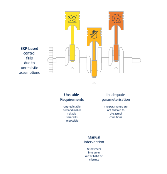
ERP systems are designed to support and largely automate planning decisions. However, this requires that demand can be forecast with sufficient accuracy and that the underlying parameters reflect the current supply situation. In practice, these very conditions are often only met to a limited extent.
On the one hand, demand in many companies is not stable enough to be reliably modelled using the system’s assumptions. On the other hand, planners regularly intervene in the proposals generated by the ERP system. Such interventions may be sensible or even necessary in individual cases, for example when additional information is available that the system is unaware of. In many cases, however, they are also made out of habit or a fundamental mistrust of automated planning.
Furthermore, in many companies, planning parameters are not maintained with the necessary consistency. Safety stock levels, batch sizes, forecasting methods or replenishment lead times are then no longer aligned with the actual operating conditions. The result is proposals that, from the users’ perspective, appear only marginally plausible.
This creates a classic vicious circle: poorly maintained parameters reduce the quality of the system’s suggestions. This low quality in turn leads to additional manual intervention. Consequently, the constant need for adjustments in day-to-day operations leaves no time to systematically improve the parameterisation. ERP-based control therefore often fails not because of the system’s fundamental capabilities, but due to a combination of unrealistic assumptions, inadequate parameterisation and inconsistent user behaviour.
3. From the problem to a structured analysis
The shortcomings described are well known in many companies. They manifest themselves in excessively high stock levels, recurring interventions in the planning process, or an overall lack of reliability in planning. Such symptoms can be observed in day-to-day operations, but they are often not systematically measurable and can therefore only be managed to a limited extent.
To analyse the causes of these problems in a structured manner rather than merely speculating about them, a clear set of key performance indicators is required. Only this provides transparency regarding how the system actually operates, what potential lies within the existing setup, and what target values are actually realistic.
4. Key performance indicators for assessing reality
A single key performance indicator is not sufficient to provide a sound assessment of a supply chain’s performance. Only by systematically comparing different key performance indicators is it possible to gain a nuanced understanding of the interplay between the system, parameters and user behaviour.
The following key performance indicators provide different perspectives on reality: the performance actually achieved, the potential inherent in the system, and a theoretical ideal scenario. Only when these are considered together does a complete picture emerge.
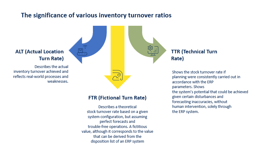
4.1 ALT (Actual Location Turn Rate)
The Actual Location Turn Rate (ALT) describes the actual inventory turnover achieved by a given unit, such as a plant or a planning level.
It reflects the actual outcome of the interaction between the ERP system, parameter settings and human intervention. This figure reflects both processes that are working effectively and existing weaknesses.
The ALT value is therefore an important starting point for any analysis. It shows where a company stands today – but says nothing about what level of performance is actually achievable or economically viable.
4.2 TTR (Technical Turn Rate)
The Technical Turn Rate (TTR) describes the inventory turnover that would result if planning were consistently carried out in accordance with the parameters currently set in the ERP system.
It thus isolates ‘system performance’ from actual usage in day-to-day operations. Differences between ALT and TTR reveal the extent to which manual interventions influence the result.
The TTR value shows the potential inherent in the existing system. At the same time, it makes it clear that this potential can only be realised if the parameters are correctly set and the planners consistently implement the system’s recommendations.
Important: TTR is based on realistic assumptions (including forecasting errors) – but using the current parameters.
4.3 FTR (Fictional Turn Rate)
Die Fictional Turn Rate (FTR) beschreibt einen theoretischen Lagerumschlag, der sich unter der Annahme perfekt zutreffender Prognosen ergeben würde.
Diese Annahme ist in vielen ERP-basierten Planungen implizit enthalten: Bedarfe treten exakt so ein wie prognostiziert, und es kommt zu keinen Störungen in der Versorgungskette. Unter diesen Bedingungen lassen sich sehr hohe Umschlagshäufigkeiten und entsprechend niedrige Bestände berechnen.
In der Praxis ist dieser Zustand jedoch nicht erreichbar. Der FTR-Wert beschreibt daher keine realistische Zielgröße, sondern eine idealisierte Referenz.
Abgrenzung zur TTR:
- TTR: reale Prognosequalität + aktuelle Parameter → realistisch erreichbares Systempotenzial
- FTR: perfekte Prognose + keine Störungen → rein theoretisches Ideal
Gerade im Vergleich mit ALT und TTR wird deutlich, wie groß die Lücke zwischen theoretischen Annahmen und realer Leistungsfähigkeit sein kann. Diese Differenz macht strukturelle Defizite in Prognosequalität, Parametrisierung und Steuerungslogik sichtbar.
5. Key performance indicators without target figures: Where the gap lies
The key performance indicators introduced earlier shed light on various aspects of reality. They help to understand where a company stands (ALT), what potential lies within the existing system (TTR) and how far theoretical ideal assumptions deviate from practice (FTR). In doing so, they create transparency – but not yet a sense of direction.
This transparency alone is not sufficient for managing the supply chain. None of the key performance indicators mentioned provides a reliable target figure against which decisions in day-to-day operations or at management level can be aligned. ALT is backward-looking, TTR merely describes the current system behaviour, and FTR is based on unrealistic assumptions.
6. Why traditional approaches are insufficient
Traditional approaches to determining target metrics in the supply chain often rely on simplified models. These include, in particular, static value stream analyses or rough estimates based on the assumption of constant inflows and outflows. However, these assumptions are at odds with the reality faced by many companies, where demand, lead times and internal processes are highly dynamic.
A key problem lies in the fact that planning decisions are influenced by a multitude of interlinked parameters. Forecasting methods, safety stock levels, batch size logic, lead times and cost assumptions do not operate in isolation, but in combination. Even small changes to individual parameters can have a noticeable impact on stock levels, service levels and costs.
For the sake of clarity, these influencing factors can be broadly categorised into several parameter groups: forecasting parameters (e.g. methods, time period, weighting), inventory parameters (e.g. safety and minimum stock levels), planning logic (e.g. MRP types and batch size methods), time parameters (e.g. delivery and lead times) and cost parameters (e.g. ordering and storage costs). In practice, these parameters are interlinked and together determine the behaviour of the supply chain.
Simplified, static calculations cannot adequately capture these interrelationships. They reduce complexity, but in doing so exclude key influencing factors. The target values derived from them are therefore either too rough or based on assumptions that do not hold true in reality.
This makes it clear that traditional approaches are not suitable for deriving a robust yet realistic target metric for supply chain management. A method is needed that takes dynamics, uncertainty and parameters into account simultaneously.
7. Approach: Dynamic Value Stream Simulation
To establish a robust basis for decision-making, a method is required that captures the real-world dynamics of the supply chain whilst taking into account the multitude of relevant parameters. This is precisely where dynamic value stream simulation comes into play.
Unlike static approaches, it works with real historical demand trends. These are used to replicate the interplay between forecasting, planning and material flow under realistic conditions. In this way, it is possible to simulate how stock levels, delivery readiness and costs actually develop under given conditions.
A key advantage is that all relevant planning parameters are brought together in a consistent model. Changes to individual parameters can be tested in a targeted manner, and their effects become visible in conjunction with all other influencing factors. This makes it possible, for the first time, to understand which settings lead to which results.
In practice, this approach is often implemented in the form of a digital twin of the supply chain. Such a digital twin realistically maps the materials, structures, parameters and decision-making logic of an ERP system. Simulations can thus be carried out without interfering with operational processes.
There are solutions available on the market that are based on ERP data and combine simulation with optimisation (e.g. DISKOVER from SCT GmbH). What matters most is not so much the specific tool as the ability to integrate dynamics, uncertainty and parametric factors.
Dynamic value stream simulation thus creates the conditions not only for evaluating planning decisions, but also for systematically improving them.
8. From Simulation to Target Metrics
Dynamic value stream simulation fundamentally broadens our perspective on the supply chain. It not only shows how the system behaves under given conditions, but also reveals the actual impact of changes to parameters and planning logic.
This creates, for the first time, a robust basis for systematically comparing and quantitatively evaluating different courses of action. Decisions are no longer made on the basis of experience or simplified assumptions.
At the same time, it becomes clear which results are realistically achievable under the given conditions and where the economically sensible balance between stock levels, costs and delivery readiness lies.
Only on this basis can a target figure be defined that can serve as a guide for managing the supply chain. Such a target figure is neither theoretically excessive nor purely backward-looking, but is derived from the actual behaviour of the system under realistic conditions.
9. The COLT value as a realistic target metric
The COLT value (Cost Optimal Location Turn Rate) describes the cost-optimal, location-specific inventory turnover rate under realistic conditions. It is not the result of a static calculation, but arises from a combination of simulation and targeted optimisation of the planning parameters.
Its central function is to provide a robust target figure for supply chain management. The COLT value translates the conflicting objectives of stock levels, costs and delivery readiness into a concrete, manageable key performance indicator. This provides, for the first time, a framework against which both operational decisions in planning and management decisions can be aligned.
In terms of content, the COLT value combines three dimensions: the inventory level and thus the capital tied up, the costs incurred (in particular ordering, storage and process costs), and delivery readiness or the targeted service level. It is crucial that these factors are not considered in isolation, but rather in their interplay under realistic demand patterns, uncertainties and system responses.
Compared with the key performance indicators considered previously, the distinctive role of the COLT value becomes clear: whilst ALT describes the past, TTR reflects the system’s current potential and FTR is based on unrealistic ideal assumptions, the COLT value defines an economic optimum that can be achieved under real-world conditions.
For practical management, the COLT value opens up several points of departure. It enables target ranges to be derived for different product groups, plants or value streams, and deviations between the actual state (ALT) and the target state (COLT) to be systematically evaluated.
The magnitude of these deviations highlights potential for economic improvement and simultaneously indicates where action is most urgently required – whether through more consistent use of the system’s recommendations or through further optimisation of the underlying parameters.
Furthermore, the COLT value can be established as a key performance indicator within the company. It serves as a basis for KPI systems, target agreements and S&OP processes, thereby linking operational planning with overarching objectives such as working capital and service levels. In this way, an analytical metric becomes a central management tool for the continuous improvement of the supply chain.
10. Practical application: What is realistically achievable
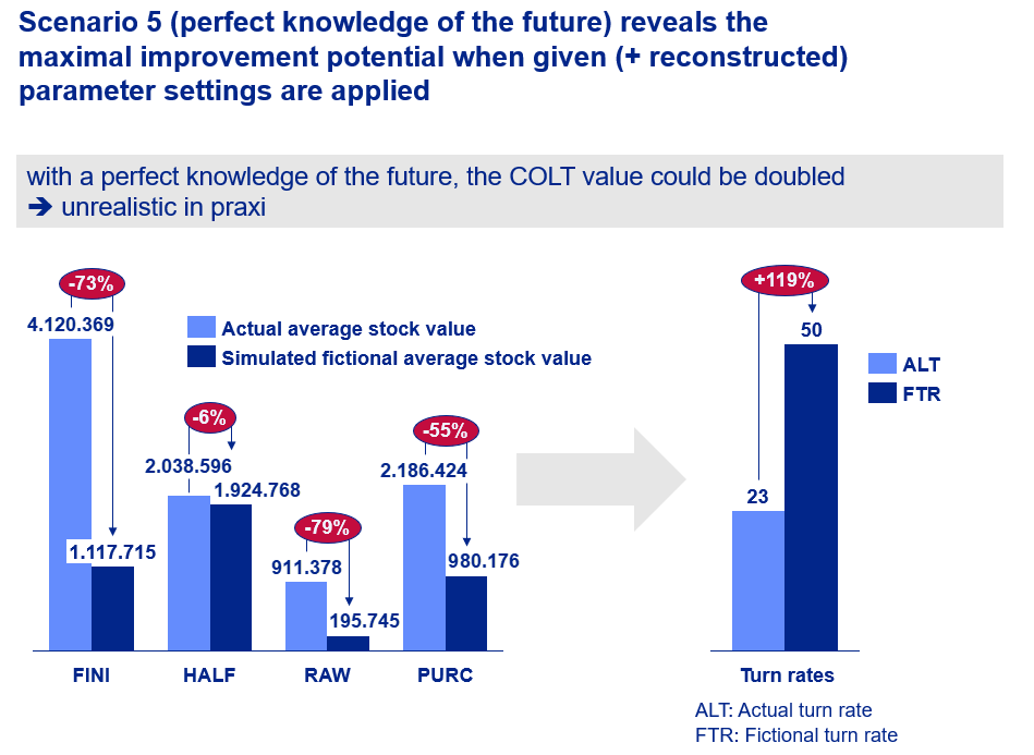
An initial simulation example at plant level illustrates just how far apart theoretical and realistic target scenarios can be. The starting point is the actual current situation, with today’s average stock levels in the material groups under consideration and an ALT value of 23.
If a simulation is carried out for the same plant on the assumption of a completely accurate demand forecast, a very different picture emerges. In this case, the calculated stock levels would be significantly reduced: by 73 per cent for finished goods, 6 per cent for semi-finished goods, 79 per cent for raw materials and 55 per cent for purchased parts. At the same time, inventory turnover would increase from an ALT value of 23 to an FTR value of 50.
It is precisely this comparison that is important in terms of content. It does not show a realistically achievable improvement programme, but rather a theoretical ideal world. The comparison thus reveals the potential that, in theory, lies within the system under perfect forecasting conditions. At the same time, it becomes clear why such figures are unsuitable as operational targets: they presuppose a level of forecasting accuracy that is unattainable in practice.
For business management, the value of such an example therefore lies not in deriving a target value, but in contextualising the theoretical maximum. Only by comparing it with more realistic simulations – for example, based on actual forecasting errors and optimised parameters – can one assess what potential for improvement can actually be realised under real-world conditions.
11. Systematically resolving conflicting objectives
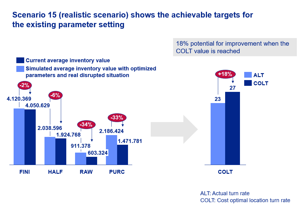
A second simulation example demonstrates the improvements that can actually be achieved under realistic conditions and with optimised replenishment parameters. The starting point is once again the current state, with the current average stock levels and an ALT value of 23.
Unlike the previous example, the simulation is based on realistic forecast inaccuracies and optimised planning parameters. It is also assumed that the planning process consistently follows the system’s recommendations and that no manual interventions take place. The result thus represents the COLT value.
Important for interpretation: The light blue bars show the current actual situation, whilst the dark blue bars represent the COLT value.
The results are significantly more moderate than in the theoretical ideal case, but are realistically achievable. Stock levels can be reduced to varying degrees depending on the material group: by 2 per cent for finished goods, 6 per cent for semi-finished goods, 34 per cent for raw materials and 33 per cent for purchased parts. At the same time, stock turnover rises from an ALT value of 23 to a COLT value of 27, which corresponds to an improvement of around 18 per cent.
12. From Project to Management Framework: ERP Performance Management
The analyses and simulations presented so far show that the performance of a supply chain can be systematically improved. It is crucial, however, that these findings are not viewed as a one-off project, but are incorporated into a sustainable management framework.
In many companies, the optimisation of planning parameters remains a one-off exercise. Parameters are adjusted once, but are not subsequently developed further in a consistent manner. Against a backdrop of changing demand, lead times and market conditions, this means that even well-tuned systems lose performance over time.
This is precisely where ERP performance management comes in. The aim is to establish the simulation and optimisation of planning parameters as a continuous process. Based on current data, parameters are regularly reviewed, adjusted and automatically reset using appropriate tools (e.g. DISKOVER).
Dynamic value stream simulation plays a central role in this process. It serves not only as a one-off analysis but as an ongoing tool for identifying the effects of changing conditions at an early stage and deriving appropriate measures. In this way, planning is gradually stabilised and simultaneously optimised for economic efficiency.
A key factor for success is integration into existing planning and control processes. The insights gained from simulation and optimisation must be incorporated into operational planning, S&OP processes and the company’s KPI system. Only in this way can a seamless link be established between analytical assessment and day-to-day decision-making.
As a result, the role of the ERP system changes: from a purely executional planning tool to an actively managed system whose performance is continuously monitored and improved. ERP performance management therefore means not only operating the supply chain, but also actively managing and developing it.
13. Conclusion: COLT as a key performance indicator for the supply chain
The COLT value bridges the key gap in supply chain management: it provides a realistic, economically sound target derived from the system’s optimised behaviour under realistic conditions. It therefore neither replaces existing key performance indicators nor operational control metrics, but provides a benchmark tailored to the specific planning and control situation.
For management, this represents a new level of quality in decision-making. Instead of retrospective metrics or theoretical target values, a robust reference is available that shows which performance level is sensible and achievable under given conditions. In the event of changes to stock targets, service levels or parameter settings, a corresponding COLT value can be determined directly, which can be used to monitor compliance with targets within the context of planning.
At the same time, the COLT value links operational planning with strategic control. It makes the effects of parameter settings, forecast quality and user behaviour transparent.
In conjunction with an established ERP performance management system, the COLT value thus becomes the key performance indicator for the supply chain. It enables not only isolated improvements, but also the continuous, systematic development of the entire value chain.
FAQ – Frequently Asked Questions
What is the COLT value?
The COLT value (Cost Optimal Location Turn Rate) describes the cost-optimal stock turnover rate for a warehouse or site under realistic conditions. It is determined through simulation and optimisation of the planning parameters and serves as a target metric for an economically optimal supply chain.
What is the COLT value used for in practice?
Excel is not a problem as a tool in itself, but rather in the way it is used:
- it creates parallel data silos
- it prevents real-time transparency
- it is prone to errors
- it hinders cross-departmental collaboration
In complex systems, this leads to systematic inconsistencies.
What is the difference between COLT and ALT?
- ALT (Actual Location Turn Rate) describes the actual stock turnover achieved.
- COLT describes the optimal stock turnover achievable under realistic conditions.
ALT shows the current status, whilst COLT shows the target status.
What does TTR (Technical Turn Rate) mean?
The Technical Turn Rate (TTR) describes the inventory turnover that would result if planning were carried out consistently in accordance with the current ERP parameters – without any manual intervention. It demonstrates the potential of the existing system.
What is the difference between TTR and COLT?
- TTR is based on the currently set parameters
- COLT is based on optimised parameters
TTR shows what is possible today – COLT shows what would be optimal.
What does FTR (Fictional Turn Rate) mean?
The Fictional Turn Rate (FTR) describes a theoretical stock turnover rate based on the assumption of perfect forecasts and smooth operations under given planning parameters. It corresponds to the value that would result if the future developments shown in the planning list of an ERP system (e.g. MD04 in the SAP system) were to occur exactly as predicted. In practice, this scenario is unattainable.
Why are traditional key performance indicators not enough?
Key performance indicators such as inventory turnover or service levels only reveal certain aspects of the supply chain. They do not provide an answer as to which performance level is economically optimal. Without a target metric such as the COLT value, management often remains reactive.
What is a dynamic value stream simulation?
A dynamic value stream simulation models the actual behaviour of the supply chain based on historical data. It takes into account forecasting errors, parameters and system responses, and enables a realistic assessment of stock levels, costs and service levels.
What is a digital twin in the supply chain?
A digital twin is a virtual representation of the real-world supply chain. It enables scenarios and changes to parameters to be simulated without affecting day-to-day operations.
How does simulation help to optimise scheduling?
Simulation makes it possible to test the effects of parameter changes in advance, taking into account the real-world constraints of practical operations. This enables the identification of optimal settings that reduce stock levels whilst ensuring delivery readiness.
Warum greifen Disponenten in ERP-Vorschläge ein?
Manual interventions often occur because:
additional information is available
there is a lack of trust in the system
or established habits are in place
These interventions can be useful, but they often lead to inefficient results.
What is ERP performance management?
ERP performance management refers to the continuous monitoring and optimisation of planning parameters within the ERP system. The aim is to ensure the long-term efficiency and stability of the supply chain.
What role does the service level play in the COLT analysis?
The service level is a key performance indicator alongside stock levels and costs. The COLT value ensures that stock levels are not minimised in isolation, but are always optimised in line with the desired service level.
How can you identify areas for improvement in the supply chain?
By comparing:
- Current status (ALT)
- System potential (TTR)
- Optimal target value (COLT)
The difference shows where and how improvements can be made.
What benefits does the COLT analysis offer businesses?
- realistic targets rather than theoretical figures
- reduced stock levels and lower capital tied up
- greater delivery capacity
- a better basis for decision-making
- continuous optimisation of the supply chain
How exactly is the COLT value calculated?
The COLT value is not calculated directly, but is determined through simulation. This process takes into account historical demand, planning parameters and target metrics such as costs and service levels, and optimises them iteratively.